Line Of Best Fit Calculator

Linear regression remains one of the most powerful statistical tools for analyzing relationships between variables. Whether you’re a student grappling with statistics homework or a data scientist analyzing complex datasets, understanding how to calculate and interpret the line of best fit is essential for making informed decisions based on data.

Understanding the Line of Best Fit

The line of best fit, also known as the regression line or trend line, represents the straight line that best describes the relationship between two variables in a dataset. This line minimizes the distance between itself and all data points, providing the most accurate representation of the underlying trend.

Why Linear Regression Matters

Linear regression serves multiple purposes in data analysis:

Predictive Power: Once you establish a reliable line of best fit, you can predict future values based on historical data patterns.

Relationship Analysis: The tool helps identify the strength and direction of relationships between variables, revealing whether they move together positively, negatively, or show no correlation.

Decision Making: Businesses use linear regression to forecast sales, analyze market trends, and optimize resource allocation based on data-driven insights.

Applications Across Industries

The versatility of linear regression makes it invaluable across numerous fields:

Financial Services: Investment analysts use regression to predict stock prices and assess market volatility based on economic indicators.

Healthcare: Medical researchers analyze the relationship between treatment dosages and patient outcomes to optimize therapeutic protocols.

Marketing: Companies examine the correlation between advertising spend and sales revenue to maximize return on investment.

Manufacturing: Quality control teams use regression to identify relationships between production variables and product defects.

The Mathematics Behind Linear Regression

Understanding the formula Y = mX + b forms the foundation of linear regression analysis, where each component plays a crucial role in defining the relationship between variables.

Breaking Down the Formula

Y (Dependent Variable): This represents the outcome you’re trying to predict or explain. Examples include sales revenue, student test scores, or patient recovery times.

X (Independent Variable): This is the predictor variable that influences the dependent variable. Examples include advertising spend, study hours, or treatment duration.

m (Slope): The slope indicates how much Y changes for every one-unit increase in X. A positive slope shows that as X increases, Y increases, while a negative slope indicates an inverse relationship.

b (Y-Intercept): This represents the predicted value of Y when X equals zero. While not always practically meaningful, it’s mathematically necessary for the equation.

Interpreting Slope and Intercept

The slope provides the most actionable insights from your regression analysis. For instance, if you’re analyzing the relationship between marketing spend and sales revenue, a slope of 2.5 means that for every additional dollar spent on marketing, sales revenue increases by $2.50 on average.

The intercept represents your baseline value. Using the same example, an intercept of $10,000 suggests that even with zero marketing spend, you’d expect $10,000 in sales revenue from other factors.

Essential Assumptions for Reliable Results

Before applying linear regression, verify that your data meets these critical assumptions to ensure accurate and meaningful results.

Linear Relationship

Your data should demonstrate a roughly linear pattern when plotted on a scatter plot. If the relationship appears curved or follows a different pattern, linear regression may not be appropriate.

Normally-Distributed Scatter

The residuals (differences between actual and predicted values) should be normally distributed around the regression line. This ensures that your predictions are unbiased and reliable.

Homoscedasticity

The variance of residuals should remain constant across all values of X. If the spread of data points increases or decreases systematically along the regression line, this assumption is violated.

Independence of Observations

Each data point should be independent of others. This means that the value of one observation shouldn’t influence another, which is particularly important in time-series data.

No Uncertainty in Predictors

The X values should be measured without error or with minimal measurement uncertainty. Significant errors in predictor variables can lead to biased results.

Our Free Line of Best Fit Calculator: Your 2025 Solution

Our advanced calculator addresses the limitations found in competing tools while providing an intuitive, comprehensive analysis platform.

Step-by-Step Usage Guide

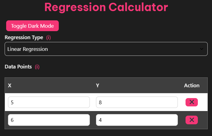
Data Input: Enter your X and Y values in the designated fields. Our calculator accepts various formats, including comma-separated values and column format for easy data transfer.

Automatic Processing: Click “Calculate” to instantly generate your regression analysis. The calculator processes your data using the least squares method for optimal accuracy.

Result Interpretation: Review the comprehensive output including the regression equation, correlation coefficient, and statistical significance measures.

Visualization: Examine the automatically generated scatter plot with the line of best fit overlay to visually assess the relationship quality.

Unique Features That Set Us Apart

Step-by-Step Guidance: Unlike basic calculators, our tool provides explanatory text for each result, helping users understand what the numbers mean in practical terms.

Instant Scatter Plot Visualization: See your data and regression line immediately, making it easy to identify outliers and assess the fit quality.

Advanced Metrics: Access R-squared values, P-values, and confidence intervals to thoroughly evaluate your regression model’s reliability.

Large Dataset Capability: Process extensive datasets efficiently, making it suitable for complex academic and professional projects.

User-Friendly Interface: Our intuitive design ensures smooth operation regardless of your statistical background.

Technical Implementation

Our calculator employs the least squares method to minimize the sum of squared errors between actual data points and the regression line. This approach ensures optimal fit while providing standard error estimates for reliability assessment.

Real-World Applications and Examples

Understanding how to apply linear regression in practical scenarios helps bridge the gap between theory and real-world problem-solving.

Financial Forecasting

Investment professionals use linear regression to predict stock prices based on historical performance and market indicators. For example, analyzing the relationship between company revenue growth and stock price movements helps investors make informed decisions.

Example: A financial analyst examining the relationship between quarterly earnings and stock price discovers that for every $1 increase in earnings per share, the stock price increases by $12 on average. This relationship, quantified through linear regression, guides investment recommendations.

Economic Analysis

Economists frequently use regression analysis to understand relationships between economic indicators and forecast future trends.

Example: An economic researcher studying unemployment rates and GDP growth finds that for every 1% increase in GDP growth, unemployment decreases by 0.3%. This relationship helps policymakers understand the economic impact of growth initiatives.

Sales Projections

Businesses rely on linear regression to forecast sales based on various factors such as marketing spend, seasonal trends, and economic conditions.

Example: A retail company analyzing the relationship between advertising expenditure and monthly sales revenue discovers that every $1,000 invested in advertising generates $3,500 in additional sales. This insight helps optimize marketing budgets.

Research and Development

R&D teams use regression analysis to understand relationships between research inputs and innovation outputs, helping optimize resource allocation.

Example: A pharmaceutical company studying the relationship between research investment and successful drug discoveries finds that each additional $10 million in R&D spending correlates with 0.8 additional successful compounds. This guides strategic investment decisions.

Educational Applications

Students and educators use linear regression to understand statistical concepts and analyze academic performance data.

Example: A education researcher examining the relationship between study hours and test scores finds that each additional hour of study correlates with a 3-point increase in test scores, helping students optimize their study strategies.

Best Practices for Accurate Analysis

Following these guidelines ensures reliable results and meaningful insights from your linear regression analysis.

Data Quality Assurance

Check for Outliers: Examine your scatter plot for data points that appear significantly different from the overall pattern. These outliers can disproportionately influence your regression line.

Verify Data Accuracy: Ensure all data entries are correct and represent the intended measurements. Small errors in data entry can significantly impact results.

Assess Completeness: Missing data can bias your results. Consider whether missing values are random or systematic before proceeding with analysis.

Statistical Validation

Evaluate R-squared: This metric indicates how much of the variation in Y is explained by X. Higher R-squared values (closer to 1) suggest stronger relationships, but don’t automatically indicate causation.

Check P-values: These help determine statistical significance. P-values less than 0.05 typically indicate that the relationship is statistically significant and unlikely to be due to chance.

Examine Residuals: Plot residuals to check for patterns that might indicate violations of regression assumptions.

Interpretation Guidelines

Correlation vs. Causation: Remember that correlation doesn’t imply causation. A strong linear relationship doesn’t mean that X causes Y; other factors might influence both variables.

Sample Size Considerations: Larger sample sizes generally provide more reliable results, but the minimum required size depends on your specific application and desired confidence level.

Practical Significance: Consider whether statistically significant results are practically meaningful in your context.